
Investor behavior drives the market’s calendar patterns
Investor behavior drives the market’s calendar patterns

Seasonality and calendar patterns exist for many markets and can become a key factor in evaluating and developing actively managed investment strategies. Taking advantage of them can improve your returns and help lower risk.
We are creatures of habit. We get up at the same time each day, drink coffee or tea, take the same train to work standing on the platform next to the same people, or drive to work and park in the same slot next to the same cars. We are uncomfortable when that pattern is interrupted.
It will not be a surprise that we invest the same way. Actually, large groups of investors buy and sell the same way. They listen to the same news and form the same opinions. They enter their orders on Monday or at the end of the day because it is convenient. Investor behavior results in many calendar patterns, from cycles of just a few days to the “Santa rally” and the presidential cycle. Some of them are reliable and can help improve your portfolio results. Other market calendar patterns may be well-known but no longer work. We’ll look at a broad range of calendar patterns and see what the statistical evidence says.
The presidential cycle
Let’s start with the presidential cycle because that seems to be at the forefront of everyone’s minds. Next year will be the third, and last, year of the cycle, if the election year is considered year one. Figure 1 shows that it is the best year of the cycle (although recently not as strong as the previous 50 years). That should be good news for investors. But this pattern is driven by government action. The incumbent party wants a strong economy to help them get re-elected and, up to recently, voters focused on how the economy directly affected them. We seem to have a shift—hopefully, a temporary one—that puts more focus on personalities. Still, the controlling party will want to emphasize how well they have improved the economy.
FIGURE 1: MARKET RETURNS DURING THE PRESIDENTIAL CYCLE (1948–2016)
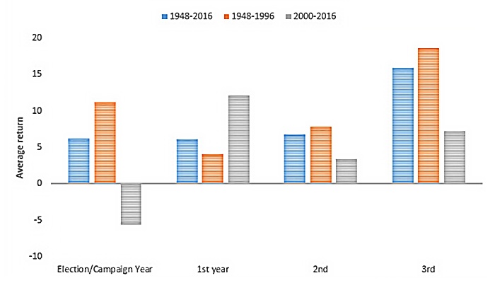
Source: Perry Kaufman, data from Commodity Systems Inc. (CSI)
Even more interesting is the consistency of those yearly returns, shown in Figure 2. The year of the election shows a wide range of profits and losses, but the third year (which will be 2019) shows nearly all gains.
FIGURE 2: RANGE OF RETURNS IN THE PRESIDENTIAL CYCLE (1948–2016)
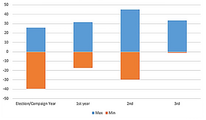
Source: Perry Kaufman, data from Commodity Systems Inc. (CSI)
To understand the variability of returns, Figure 3 shows the returns for each year before the election year, what we call the third year. The last three are not looking as good, but the risk has historically been minimal.
FIGURE 3: YEAR-BY-YEAR RETURNS FOR THE 3RD YEAR OF THE PRESIDENTIAL CYCLE
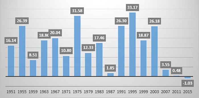
Source: Perry Kaufman, data from Commodity Systems Inc. (CSI)
The Santa rally
Yes, there is a Santa.
If we focus only on December, knowing that the holiday shopping season now generally starts before Thanksgiving, we can see that returns from 1950 through 2017 have been consistently positive—at about an 80% rate (Figure 4). Even in 1987, following the “crash,” December was a strong month. It must be the Christmas spirit!
FIGURE 4: SPX DECEMBER RETURNS (1950–2017)
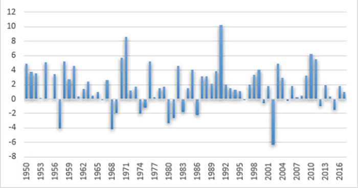
Source: Perry Kaufman, data from Commodity Systems Inc. (CSI)
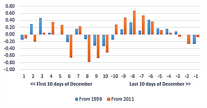
However, a Santa rally doesn’t mean that prices are higher every day. In Figure 5, the average returns are shown for the first and last 10 trading days of December. We see that the month starts out strong, sags in the week before Christmas Day, and then rallies again right around the holiday. The last two trading days of the year show average losses, perhaps because many market participants are not at work or buyers try to forget what they spent during the holidays!
FIGURE 5: SPY AVERAGE RETURNS FOR THE FIRST AND LAST 10 TRADING DAYS OF THE MONTH
Source: Perry Kaufman, data from Commodity Systems Inc. (CSI)
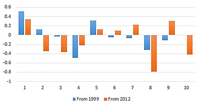
What happens in January? Optimism or buyers’ remorse? Figure 6 shows that there is usually buying on the first day of January, but the next nine days show no particular pattern.
FIGURE 6: SPY AVERAGE RETURNS FOR THE FIRST 10 TRADING DAYS OF JANUARY (1999–2016)
Source: Perry Kaufman, data from Commodity Systems Inc. (CSI)
How do we interpret that in 2018? The economy is good (although tired), unemployment is at an all-time low, corporations have a recent tax advantage, and buyers should be in a good mood. We would expect that to result in a normal holiday pattern, but the following section, “As January goes …,” should help explain it.
As January goes …
There’s good news, and there is good news. First, the good news!
Fourteen of the 18 years from 2000 through 2017 were higher in December than at the end of January in that same year, regardless of how January closed. That’s 77.7% of the years. Therefore, the chances of an annual gain after a higher January are pretty good. During those 18 years, eight had a higher January close, and six of those closed the year higher than at the end of January. That’s 75%, about the same as the average year.
Therefore, “As January goes …” is basically the same as “No matter how January goes …”
However, the years with a higher January outperformed the market during the rest of the year. The average return for the remainder of those years with a higher January was 10.1%, compared to the overall annualized rate of return of 6.4%. Then the January effect added 3.7% per year. We can definitely say “as January goes,” so goes an extra profit.
But only eight of the past 18 years posted a higher January, and most investors would like something more consistent.
“Sell in May and go away”—but for how long?
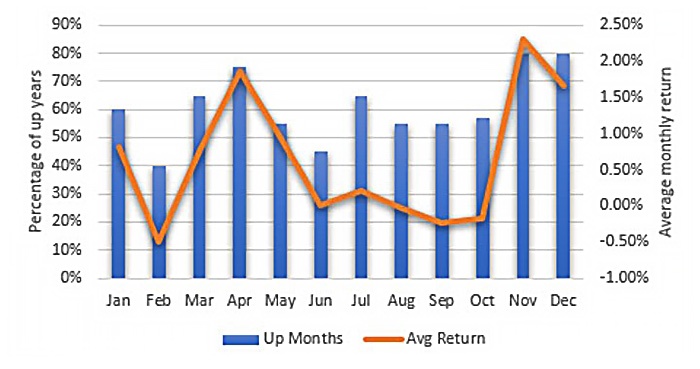
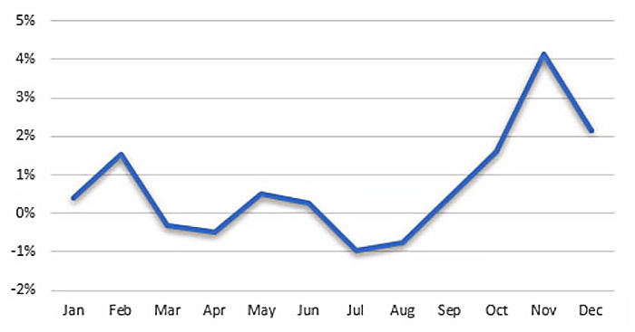
It’s true that the summer months have low volume. This is partially because investors (both professional and retail), much like everyone else, go on vacation. To avoid having to monitor the market every day, they close out or deleverage their holdings. Figure 7 shows that if you sold at the end of May during the period from 1998 through 2017, you would have (1) missed what are generally the lowest monthly returns of the year and (2) missed the months with generally the lowest percentage of positive years. Waiting until the end of October to re-enter is usually the best time.
While the upward bias of the stock market shows that the period of July through October yields positive returns more than 50% of the time, the average returns hover near zero for the period studied—keeping your positions open during those months only adds risk. As we’ve seen this year, October combined high volatility with low returns. Perhaps that’s caused by investors’ behavior. If investors worry about the volatility, they tend to react quickly to news, and that adds further to the volatility.
FIGURE 7: SPY SEASONALITY BY MONTH (1998–2017)
Source: Perry Kaufman, data from Commodity Systems Inc. (CSI)
Seasonality for corn, homebuilders, airlines, and retail sectors
While the previous patterns are based on investor and consumer behavior, they do not represent what we would call true seasonality. Seasonality is a basic factor in price movement, and it’s always there even if it’s not obvious. Sometimes it can be overwhelmed by other economic or political events, but it is still affecting prices. A single extreme good or bad year can also make the seasonal pattern look different. To find a reliable pattern requires looking at the returns, then confirming those returns with the frequency, or consistency, of it occurring each year. It’s easier to show with an example.
Seasonality is fundamental to commodities such as corn and wheat, which are planted and harvested based on the time of year. But many stocks are seasonal, including those that have a business based on tourism or dependent on commodity input. Airlines, hotels, food processors, and even bank loans can be seasonal. Homebuilders and their suppliers are more active starting in the spring in the Northern Hemisphere. Seasonality affects a wide swath of our economy. Even the S&P has a seasonal pattern, as we saw in Figure 7.
Corn
Let’s start with the basics. Corn is the largest U.S. crop and mostly used for cattle, hogs, and chicken feed. It is not the corn that you buy in the grocery store for your barbecue. It is high protein, high starch, low sugar, and engineered for feed. Corn is planted around May and harvested starting in September. Its consumption is mostly domestic, so it should have a clear seasonal pattern.
The easiest way to find seasonality is to examine the average percentage of positive yearly returns (by month) for the period studied. It avoids any complication for prices that start low and move much higher. (This methodology can also be used for stocks and sector ETFs.)
If we do that for corn, Figure 8 shows that there is a clear seasonal pattern that has not changed in the past 10 years. The lows are at the September harvest when most corn comes to market and depresses prices. Prices quickly rebound to include the cost of storage and then remain higher until the new crop is planted.
FIGURE 8: SEASONALITY OF CASH CORN PRICES (1978–2018)
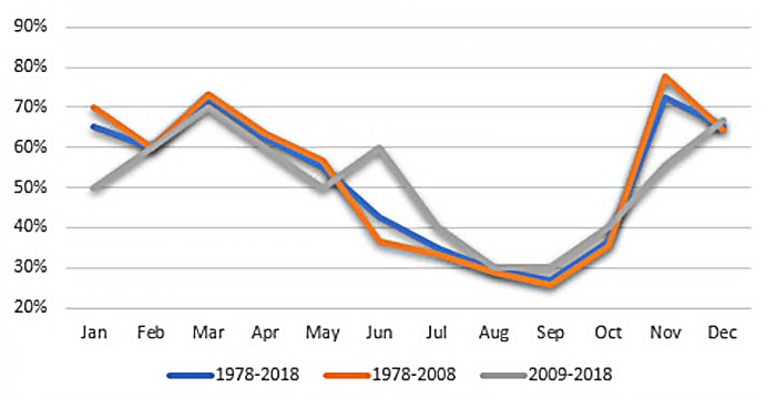
Note: Seasonality using the percentage of years when corn prices were higher, by month.
Source: Perry Kaufman, data from Commodity Systems Inc. (CSI)
Seasonality in stocks
Food processing
Is there seasonality in stocks as predictable as corn? Let’s start with an agricultural company, Archer Daniels Midland (ADM), a food processor and soybean crusher. Soybeans have a similar crop season to corn, only a little shorter. Figure 10 shows the seasonal pattern for ADM, using average yearly returns by month, declining from March through August, and then rising after harvest, much the same as corn. Based on these returns, you would favor holding ADM long from October through December and short from the end of February through July.
FIGURE 9: ARCHER DANIELS MIDLAND AVERAGE RETURNS BY MONTH (1990–2018)
Source: Perry Kaufman, data from Commodity Systems Inc. (CSI)
Airlines
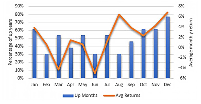
While airlines would like to emphasize business travel, which is steady throughout the year, the end-of-year travel dominates their returns as it does for retail. Figure 10 shows the average yearly returns by month. You would be wise to avoid holding American Airlines (AAL) from February through July. The likelihood of October through January showing a profit varies from 60% to 80% for the period from November 2005 through October 2018.
FIGURE 10: AMERICAN (AAL) AVERAGE RETURNS BY MONTH
AND FREQUENCY OF HIGHER RETURNS
Source: Perry Kaufman, data from Commodity Systems Inc. (CSI)
Home construction
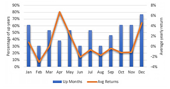
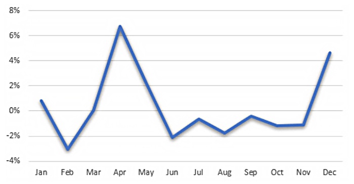
We expect housing to be another seasonal sector. Looking at leading homebuilder D.R. Horton (DRH) in Figure 11, we see that April and December have big gains, offsetting most other months, which show small average losses. But a closer look at April (Figure 12) shows that the spike was the result of a single year, 2009. The other years from 2006 through 2018 show a slightly downward April pattern.
What is clear from the DRH pattern is that one month in one year (April 2009) can create what some will interpret as a “seasonal rally,” while it was simply a data outlier. For a true seasonal pattern, we need consistency. That can be found in the percentage of up years, shown as the bar chart in Figure 11. Here we see that April only had a 40% chance of posting a profit, which is inconsistent with the size of the average yearly gain for April. Instead, we should look to December and January for the best results.
FIGURE 11: D.R. HORTON (DRH) AVERAGE RETURNS BY MONTH WITH FREQUENCY OF UP YEARS
Source: Perry Kaufman, data from Commodity Systems Inc. (CSI)
FIGURE 12: D.R. HORTON (DRH) RETURNS FOR APRIL (2006–2018)
Source: Perry Kaufman, data from Commodity Systems Inc. (CSI)
Sector SPDR Patterns
One might expect that returns for sector SPDRs as a group would, over time, look the same as the overall market pattern seen in the SPY seasonality. But there are also idiosyncrasies, as seen in Table 1. Not surprisingly, the December column is profitable for all, though Energy and Utilities lag other sectors. Retail is strong in April and September (the spring and fall selling seasons), and December is (also not surprisingly) the big month for retail. There are no green boxes (the best returns) for any sectors during the summer months, and January through March have no outstanding values except for health care in January, perhaps the results of new and renewing members of health-care plans and the height of the cold-and-flu season.
TABLE 1: HEAT MAP OF SECTOR SPDRS (1998–2018)
Frequency of a higher return. Green shows the highest returns, red the lowest.
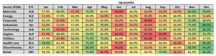
Source: Perry Kaufman, data from Commodity Systems Inc. (CSI)
When we look at the average returns by sector and month in Table 2, April, November, and December stand out. We then have a combination of a high chance of a profit and a good average return. It’s obviously a good thing for investors to have history on their side.
TABLE 2: HEAT MAP OF SECTOR SPDRS (1998–2018)
Average monthly returns
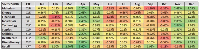
Source: Perry Kaufman, data from Commodity Systems Inc. (CSI)
(Editor’s note: Major sector changes were introduced by the Global Industry Classification Standard, or GICS, in September 2018—changes that resulted in 1,000 companies being reclassified globally. See Proactive Advisor Magazine’s October 2018 article, “Understanding the nuances of sector fund exposure.”)
The two most important components of seasonality
To take advantage of seasonal patterns, you need two criteria: a positive average return for the months that you trade, and a high likelihood that those months will produce good returns. A lower frequency means that one year was an outlier and might not represent a dependable pattern. Both returns and frequency can be analyzed using a spreadsheet, with monthly data downloaded from any number of sources. Seasonality exists for many markets and can become a key factor in evaluating and developing actively managed investment strategies. Taking advantage of it can improve your returns and help lower risk.
The opinions expressed in this article are those of the author and do not necessarily represent the views of Proactive Advisor Magazine. These opinions are presented for educational purposes only.
 Perry Kaufman is a financial engineer specializing in algorithmic trading. He is best known for his book, “Trading Systems and Methods,” (fifth edition, Wiley, 2013) and recently published “A Guide to Creating a Successful Algorithmic Trading Strategy” (Wiley, 2016). Mr. Kaufman has a broad background in equities and commodities, global macro trading, and risk management. Find more information at his website: www.kaufmansignals.com
Recent Posts: