Can managing market volatility really be simple?

A recent study from Yale University says your emotions may be right: avoiding risk in periods of high market volatility can be a winning strategy

This paper garnered a fair amount of media attention. One suspects it was because this seemed to be a strong academic support point for portfolio risk management and some of the underlying theories favored by proponents of actively managed strategies. In a world where advocates of a buy-and-hold philosophy have grown more emboldened with each year of the current bull market, this paper is certainly worth close examination.

Overview of the ‘volatility managed’ strategy and its results

The strategy boils down to two somewhat tongue-twisting rules:

1. Compute realized volatility for a given month for a given factor by taking the square root of the variance of the preceding month’s daily returns.
2. Construct portfolios by scaling each factor by the inverse of its realized variance, increasing or decreasing exposure at the start of each month based on the prior month’s realized variance.

In an interview on CNBC’s Trading Nation in March 2016, co-author Muir more simply stated the fundamental finding of the study:

Moreira and Muir also maintained that since the strategy simply involves consulting a standard measure of volatility and trading once a month, an average investor could pursue such a strategy for themselves.

Before the average investor attempts the strategy, however, a few reality checks need to be made.

In studying volatility, the authors found that there is little relation between lagged volatility and average returns, but there is a strong relationship between lagged volatility and current volatility. Realized volatility for each factor strongly predicts future volatility, but doesn’t predict the factor’s future returns, they maintain. As a result, the widely held belief that in exchange for higher risk, investors are rewarded with higher returns doesn’t hold true.

“The widely held belief that in exchange for higher risk, investors are rewarded with higher returns doesn’t hold true.”

If the investor isn’t rewarded for taking on greater risk, the prudent move should be to minimize risk exposure. Because large market losses tend to happen when market volatility is high (e.g., the most recent financial crisis of 2007–9), the strategy avoids these periods to the greatest degree possible. In periods of lower market volatility, results tend to be identical to a fully invested buy-and-hold strategy.

Based on the “volatility managed” strategy, the authors calculated that $1 invested in the “market” in 1926 would yield around $20,000 by 2015, versus about $4,000 for a buy-and-hold strategy. The following chart from the paper illustrates the gains on a logarithmic scale.

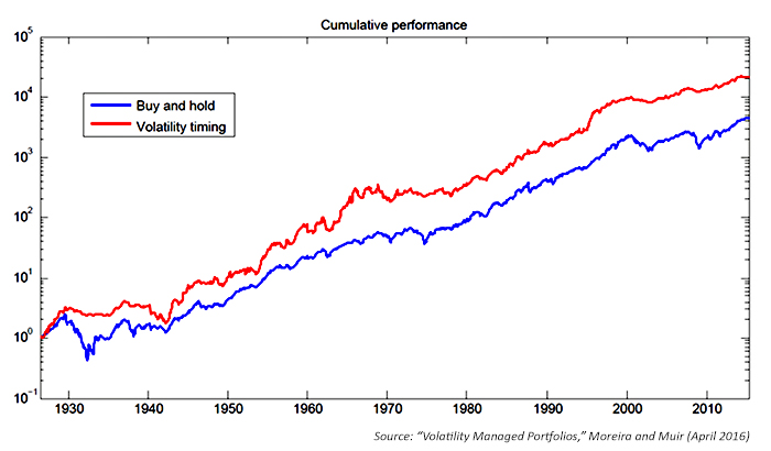
Lengthy investment periods such as this always pose the question of whether or not a fortuitous “early call” gave the strategy enough momentum that compounding kept it in the lead. The authors address this issue to some degree through the use of log scale and by analyzing the mean-variance portfolios over three 30-year subsamples (1926–1955, 1956–1985, and 1986–2015). They found stronger, more significant alphas in the first and third period and weaker results in the middle period, when volatility varied far less.

Is the study viable in the ‘real world’?

Moreira and Muir spend extensive time analyzing the significance of their results, referencing other financial studies, analyzing alphas and betas and Sharpe ratios, and examining the potential effect of leverage and hedging. They test the strategy across market, value, momentum, profitability, return on equity, and investment factors in equities, finding that volatility timing produces large utility gains and benefits both short- and long-horizon investors. The strategy is contrary to conventional wisdom because it takes less risk in recessions and crises yet still earns high average returns. But they still haven’t answered a very important question: Can their results be replicated in an actual investment portfolio?

The “given factor” cited in the investment rules is the type of portfolio being analyzed based largely on factors first developed by Eugene Fama and Kenneth French when they both were at the University of Chicago’s Booth School of Business. These well-known factors (at least in academic circles) attempt to better measure market returns beyond the structure of the capital asset pricing model (CAPM).

• In the original Fama-French three factors, Mkt represents the return of the total stock market.
• SMB (Small Minus Big) is the average return on the three small portfolios minus the average return on the three big portfolios.
• HML (High Minus Low) is the average return on the two value portfolios minus the average return on the two growth portfolios.
• Mom is the average return on the two high prior return portfolios minus the average return on the two low prior return portfolios.
• RMW (Robust Minus Weak) is the average return on the two robust operating profitability portfolios minus the average return on the two weak operating profitability portfolios.
• CMA (Conservative Minus Aggressive) is the average return on the two conservative investment portfolios minus the average return on the two aggressive investment portfolios.

Dartmouth professor Kenneth French maintains data on the factors, but actually trading the factors raises serious issues of practicality.

See Related Article: The volatility cycle

The factors tested in the paper fail to wholly meet the standard for actual in-market implementation. The most well-known investment vehicles that use the Fama-French factors are called the DFA funds (from Dimensional Fund Advisors), which are offered through selected advisors and not directly available to the public. Ironically, these funds also discourage trading frequency, which the volatility strategy requires to some degree. Replicating the factors through stock baskets would be difficult at best. The study assumes modest trading expenses, but the scale of trading required to replicate the whole stock market, to say nothing of the capital requirements, makes these costs questionable. No provision is made for the cost of managing the strategy.

One of the more practical applications of the volatility management concept is found in the study’s appendix, which is “not intended for publication.” Here the authors look at the effectiveness of applying their strategy to 20 different country indexes, with the provision that they be members of the Organization for Economic Co-operation and Development (OECD). The average change in Sharpe ratio is 0.15 and the value is positive in 80% of cases, they report. Regrettably, no time frame is provided for the data.

These questions need to be addressed before an investor puts the strategy into actual use:

• Does the strategy work with available investment vehicles such as index mutual funds, ETFs, or individual stocks?
• Is there a difference in its effectiveness with different indexes and asset classes?
• What are the drawdowns?
• Does the strategy perform consistently over shorter time periods of 5, 10, or 20 years?
• What happens when the strategy is tested against rolling 5-, 10-, and 20-year time periods?
• How often does the strategy trade over a typical year?
• How will this frequency of trading affect expenses?

This is basically an academic paper written by academics for academics, quoting all of the right academic sources and using academic measures of the market. As practical investment advice, it has a lot of blanks in the data.

There is, without question, a direct correlation between volatile market conditions and nervous investors. When portfolio values gyrate violently, media coverage becomes more intense and a vicious cycle often begins to feed on itself. Commentators strive to explain away price changes and investors start to worry, and with good reason. Equity indexes have historically experienced their greatest losses during periods of high market volatility.

The results of Moreira’s and Muir’s study illustrate once again the importance of understanding market volatility’s impact on an investment portfolio. But before one implements a strategy based on simply avoiding volatility, as active managers well know, the approach needs to be tested using investment vehicles readily available to the investor and over time frames more realistic for an investment approach. Understanding historical drawdowns and how the strategy works in different market conditions helps clients not only understand the strategy, but also to stay with it for the long term.