
Low volatility—high returns?
Low volatility—high returns?

What offers a better opportunity for investment returns: low-volatility or high-volatility markets?
During the past year, there have been two important publications on this topic that have received attention in the financial community: “Volatility Managed Portfolios,” by Alan Moreira and Tyler Muir (Yale School of Management, June 17, 2016), and “The Volatility Cycle,” by Charlie Bilello of Pension Partners (republished by Proactive Advisor Magazine, May 18, 2016).
Moreira and Muir state in their academic paper’s abstract, “Managed portfolios that take less risk when volatility is high produce large alphas, substantially increase factor Sharpe ratios, and produce large utility gains for mean variance investors.”
Mr. Bilello writes in his article, “In reality, while markets are highly efficient, they are not perfectly efficient, and there are certain market anomalies that violate the laws of the CAPM [capital asset pricing model]. One of these anomalies, known as the ‘low-volatility effect,’ argues that portfolios of low-volatility stocks tend to produce higher risk-adjusted returns than portfolios of high-volatility stocks. Lower risk with higher returns sounds too good to be true, but the evidence at this point is overwhelming.”
Both publications present well-researched and compelling arguments. The trick is to convert these concepts into real investing strategies that can be implemented on a consistent basis, in all types of market conditions.
It can be both, but it is almost always high volatility.
Price movement during low-volatility periods tends to be very orderly, until it isn’t. One type of low volatility occurs when investors are just not particularly interested in stocks or futures markets and trading volume tends to fall off. In this case, low-volatility markets would usually be accompanied by a sideways drift in prices.
This behavior can be particularly true for commodities. When the price of corn is below the cost of production, investors and traders lose interest. Producers don’t want to sell at low prices and, without any expectation of a rally, prices just meander.
However, strong upward price trends can also be associated with low-volatility markets. Unfortunately, in these cases, low-volatility markets over extended time periods have throughout history also foreshadowed some of the most violent and swift market downturns. We have all heard terms such “market euphoria” and “bubbles bursting.” Investor sentiment becomes overheated, markets overbought, and the last investors into the market are often those left with the most dramatic losses. Relatively low volatility in this sense can be a powerful contrary indicator of overvalued markets with exhausted buying power.
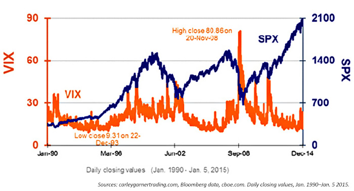
Analysis of daily Bloomberg data by the CBOE from Jan. 1, 2000, to Sept. 28, 2012, showed that the VIX moved in the opposite direction of the S&P 500 about 80% of the time. This makes strong intuitive sense and was probably learned in “Investing 101.” When markets are rising, the VIX falls. When markets are dropping, the VIX rises. The key is being able to make active and tactical course changes in one’s trading strategy when a truly discernable shift in market sentiment, investor flows, and the technical trend is beginning to take shape.
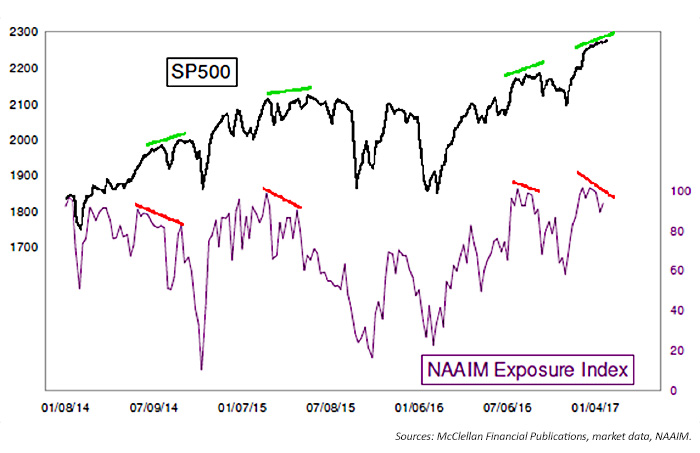
The financial author and analyst, Tom McClellan, recently constructed an interesting historical chart showing the relationship of the S&P 500 to the reported equity exposure levels of advisors and investment managers who self-identify as “active managers” (Figure 2). These individuals are part of an ongoing survey conducted by the National Association of Active Investment Managers (NAAIM) of its membership. It is a very reasonable assumption that the managers who are queried as part of the NAAIM Exposure Index are primarily trend followers who try to stay out of the way of market downturns and high-volatility periods.
NAAIM says, “The primary goal of most active managers is to manage the risk/reward relationship of the stock market and stay in tune with what the market is doing at any given time.” As Figure 2 shows, these particular active managers have been doing a pretty fair job of reducing market exposure prior to and coincident with market downturns and periods of higher volatility over the past few years.
When your portfolio volatility drops below 12% (the annualized standard deviation of the rolling returns), you increase your positon size. When it goes over 12%, you reduce your size. When you see the adjusted returns, there is a large increase during the low-volatility periods and a small decrease during the high-volatility periods. By reducing position size during high volatility, you lose a small amount of return in exchange for a large reduction in risk. So, if you are willing to give up a little return, you gain overall.
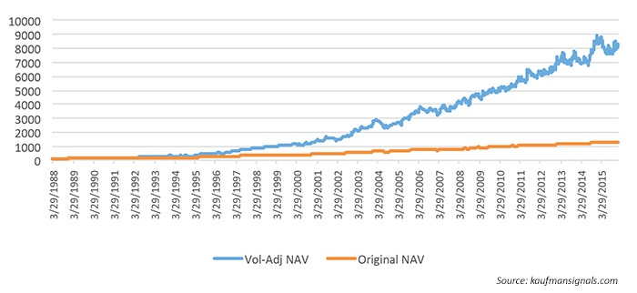
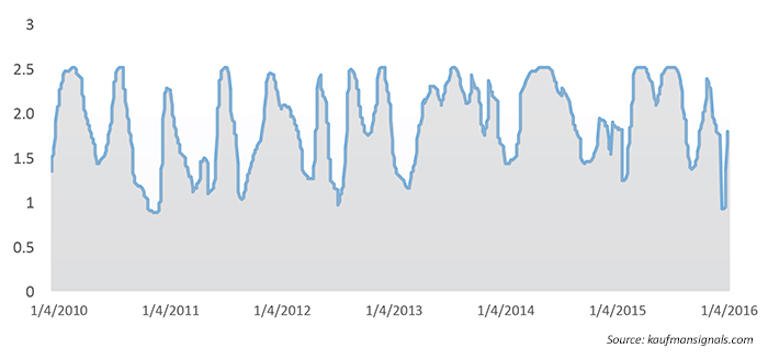
Figure 3 shows a sample Global Macro Futures Portfolio, from 1988 to 2016, which trades the same markets (about 45) all the time. Without volatility adjusting, the portfolio volatility is about 5%; after volatility adjusting, it is slightly higher than the target volatility of 12%. Adjustments to the position sizes are made based on a 20-day average true range. Note that the adjustment factor, applied to the original returns, is above 1.0 most of the time, indicating that it is increasing leverage. Put another way, the initial NAVs are leveraged up based on a volatility factor that tries to keep the returns at about 12% annualized volatility.
Another methodology has some advocates and addresses volatility a little differently. In order to decide that volatility is low, we look at a defined past period and decide if today’s volatility is in the lowest 20% of that period. If so, the portfolio or trading methodology is leveraged up.
The rules and calculations for this methodology using the S&P 500 (SPY ETF) can get as complicated as one wants, but here is a simplified version:
- Calculate the daily SPY returns in the usual way: P(t)/P(t-1) – 1, where t is the current day.
- Choose a rolling period to calculate the volatility. I favor 20 days because that provides enough time to be responsive to market changes and corresponds to the calculation period for options implied volatility.
- Find the maximum and minimum volatility over the same 20-day period.
- If we want to set the threshold (T) at 20%, then T = 0.20 x (maxvol – minvol) + minvol
- If today’s volatility is T or lower, we trade the entire investment. If not, we trade 50% of the investment.
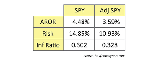
(AROR= annualized rate of return, Risk = annualized volatility, Inf ratio= information ratio)
However, this trading methodology can be significantly enhanced by changing the volatility threshold to 75%. By that, I mean trade all of the strategy investment unless the volatility is in the upper 25% of a given time period. That means we’re eliminating high volatility more than we are emphasizing low volatility. We are also using more of the investment more of the time.
The results are shown in Table 2. The adjusted returns are about 0.5% better annualized, and the information ratio is 0.36 instead of 0.30. So, we get higher returns and lower risk! Just what the doctor ordered. In looking at backtested results during the credit crisis of 2008, the maximum drawdown for this methodology was at 43%, versus a non-volatility-adjusted SPY drawdown of 51%. With some further refinements of the methodology, this still-too-high drawdown could likely be made far more favorable.
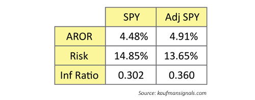
(AROR= annualized rate of return, Risk = annualized volatility, Inf ratio= information ratio)
The overall point is demonstrated in the data: avoiding the highest volatility periods can represent a tactical, active strategy that delivers better returns, lower risk, and less severe drawdowns during the worst market years.
To my way of thinking, reducing high volatility is a win-win situation. High volatility means high risk, even when it does not manifest itself in the market. My experience is that the returns during high-volatility periods do not come close to justifying the risk.
A low-volatility trading strategy, especially one that incorporates leverage, can be a tactical approach to the markets with many benefits. The very high returns of a blockbuster market year may not be attained, but, in general, more consistent, lower-risk returns can be achieved through different market cycles and a variety of volatility environments.
 Perry Kaufman is a financial engineer specializing in algorithmic trading. He is best known for his book, “Trading Systems and Methods,” (fifth edition, Wiley, 2013) and recently published “A Guide to Creating a Successful Algorithmic Trading Strategy” (Wiley, 2016). Mr. Kaufman has a broad background in equities and commodities, global macro trading, and risk management. Find more information at his website: www.kaufmansignals.com