No matter where markets are in the long-term cycle, risk is always present for all asset classes. Frequent evaluation of portfolio allocations and market exposure—and using tools such as volatility stabilization, trend following, and leverage—can significantly help in reducing portfolio risk while improving risk-adjusted returns.

We each see the opportunities in equities in our own way. Many of us expect the S&P 500 to keep going up, even with some nasty drawdowns. But it remains the real source of growth for most investors. We also see Treasury bonds as safe but with far less opportunity. The combination of stocks and bonds has been the backbone of conservative investment policy and is likely to remain that way.

We can get a recommendation to buy a stock because it is undervalued, the company has a lot of cash, promising new management, a pending product, and so on. While the availability of information and the speed of access has to some degree “democratized” investing, it has resulted in an era where the way we make investment decisions has become more complex and it is more difficult to resolve all of the information in a nice, neat package. However, we have also found that using ETFs can simplify the way we implement financial decisions. Importantly, ETFs can allow us to vary the leverage in our portfolios, much the same as using futures. This has been, and will continue to be, very valuable.

No matter how we choose to use the market, we are exposed to volatility and increasing globalization. Many investors continue to apply traditional portfolio allocation methods and little in the way of risk control. Every once in a while, we need to review those norms.

See Related Article: Let’s be realistic about drawdowns

One of the basics of investing is to hold some combination of equities and bonds. They offer critical diversification. When equities are rising in a good economy, interest rates tend to rise to temper the growth. When equities fall sharply, investors run to the safety of bonds, driving yields down. Then we need to be long equities and short yield. Shorting yield can be accomplished through being long bond futures (US/ZB) or long a bond ETF (TLT or BND). Neither should be a problem for many retirement accounts, which require long-only positions, though some retirement accounts may have limited or no access to futures.

We have always accepted the practice that a portfolio of 60% stocks and 40% bonds was right for an investor still at the age where income was flowing. It was somewhat of a surprise when, in the fall of 2019, Bank of America declared “the death of the 60-40 portfolio,” claiming that bond yields were too low. They argued that it was too risky to buy bonds and that stocks often yield more than bonds. They avoided the obvious point that stocks are also risky and that in an economic downturn, which does happen, a portfolio heavily weighted to stocks would be very risky. The stock yield cannot make up for the decline in price.

However, it still makes sense to hold both stocks and bonds. What I believe has changed is the percentage of equities and bonds that you should be holding. The “traditional” portfolio mix is to have 60% equities and 40% bonds when you’re young and increase the percentage of bonds as you get older. Let’s examine the result of using a 60-40 mix.

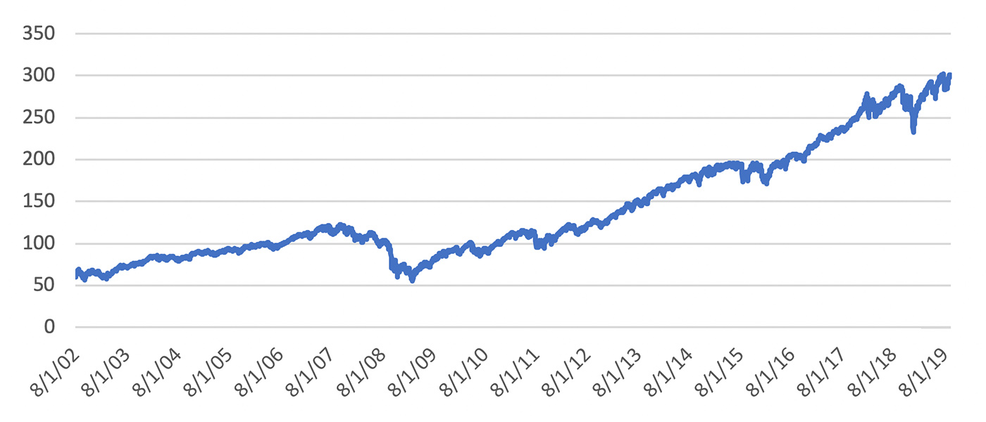
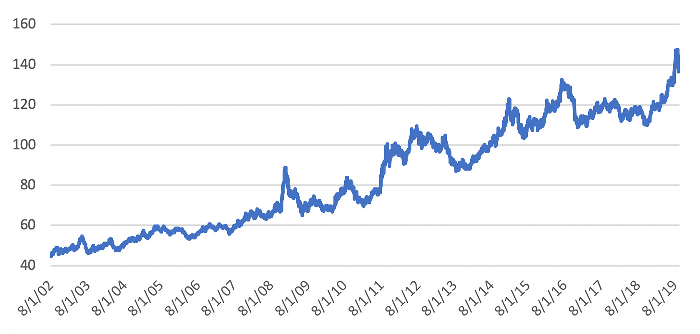
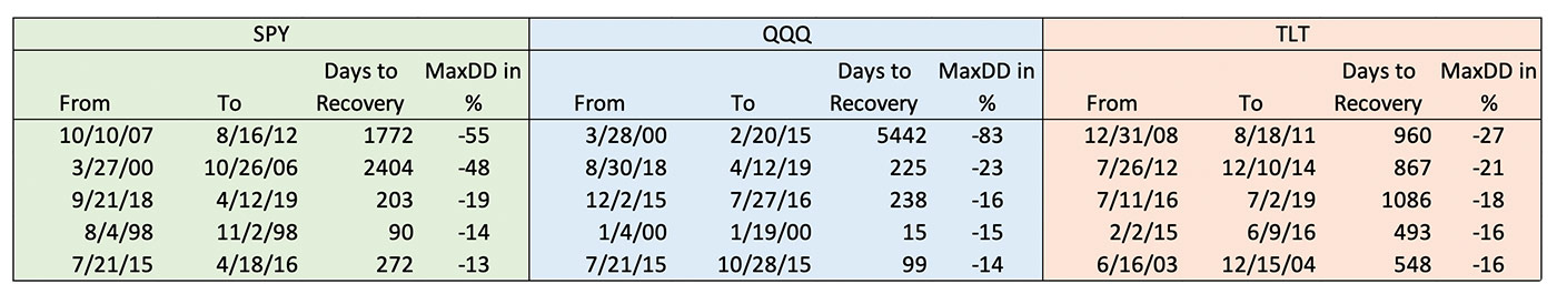
We start with SPY (S&P 500 Index ETF) and TLT (20+ Year Treasury Bond ETF) from 2002 when TLT started trading. Figures 1 and 2 show the price history. While they are both clearly up, there are some significant drawdowns. Had we gone back to include 1987 and 2001, there would be other large drawdowns. Table 1 shows the five largest drawdowns for SPY and TLT from the inception of the trading of these vehicles. For further comparison purposes, Table 1 also shows drawdown results for QQQ (NASDAQ 100 Index). (Note: Returns are indexed, not actual prices.)

Source: Market data, P. Kaufman

Source: Market data, P. Kaufman

Source: Market data, P. Kaufman

The reason for showing these drawdowns is to help understand why some investors cannot stay with a program—at some point, the stress usually becomes too much. A drawdown of 83% in QQQ would certainly discourage investors, and a recovery that lasted 15 years would be hard to rationalize. A drawdown of 55% in SPY and a five-year recovery would be nearly as bad, given the large percentage of investor assets dedicated to the S&P 500. (Just ask the investment managers at many private and public pension funds.) It is important to manage client funds so that this doesn’t happen.

The most important lesson that came out of the financial crisis of 2008 is to pay more attention to risk. Risk is volatility and drawdown.

Note: Indexed return profiles, starting at 100.

Source: Market data, P. Kaufman

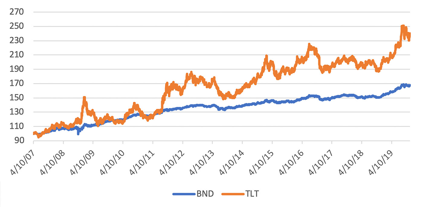
While TLT had an annualized return of 7.07% from 2007, BND returned only 4.16%. But then, there is the risk. TLT had a risk of 14.5% while BND was 4.44%, nearly 70% lower. If we judge the value by the return-risk ratio, TLT was 0.48 and BND was 0.93. Again, BND had a much smoother return. The maximum drawdown for BND was 9.3%. However, we should not forget that BND seeks to track the performance of a broad, market-weighted bond index, while TLT is equivalent to the raw prices of the Treasury 20+ year bond. BND has a much smoother path than TLT, but it also has a lower return profile.

Only the investor, financial advisor, or portfolio manager can know how much risk is acceptable, but given any risk preference, there is usually an ETF that will satisfy the need. The immutable fact is that the higher the return, the higher the risk.

We must first ask ourselves if the traditional balance of 60-40 is still the best. By “best” we mean the highest return-risk ratio, which we call the information ratio (IR), which satisfies an investor’s risk preference.

For those who prefer statistics, the ideal portfolio allocation is the point on the efficient frontier where the line from the risk-free return (on the left axis) touches the curve formed by the extreme points of portfolio risk or return, which form a U-shaped curve pointing to the left, shown in Figure 4. However, some investors will opt for a higher return with a higher risk. The best choice for them will still be on the efficient frontier but further to the right.

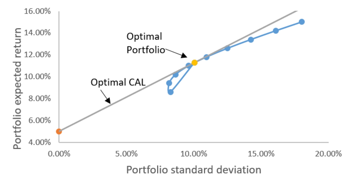
Note: CAL is the capital allocation line, and the point on the left axis is the risk-free return.

Source: Corporate Finance Institute

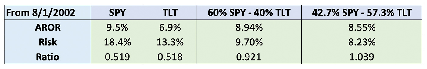
Source: P. Kaufman, data starting 8/1/2002

While the returns are only 4.5% lower for the higher allocation to bonds, the risk using the larger bond allocation is more than 15% lower. The combination gives a much better return-risk ratio. And while bonds have risk, it is far lower than anything we have seen in the 2008–2009 S&P 500 decline, or the 2000 collapse of NASDAQ (as represented via QQQ).

(Note that a similar comparison of stocks and bonds using futures shows a greater improvement due to leverage.)

If an investor or financial advisor expects 2020 to be more volatile, which seems to be the forecast, then more bonds and fewer stocks would likely make for a better portfolio allocation as a base starting point for these two asset classes. Further diversification among other asset classes also makes sense for most investors, as determined by their financial-planning objectives and longer-term investment plan.

Source: Market data, P. Kaufman

Source: Market data, P. Kaufman

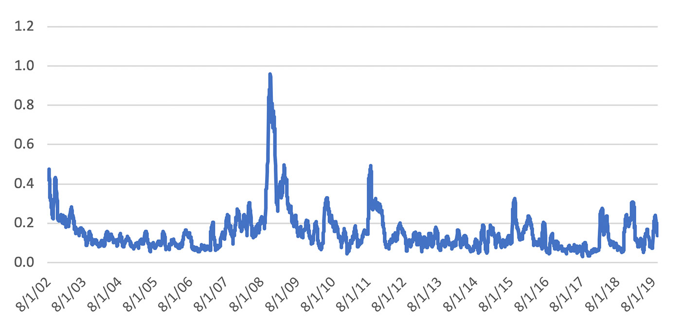
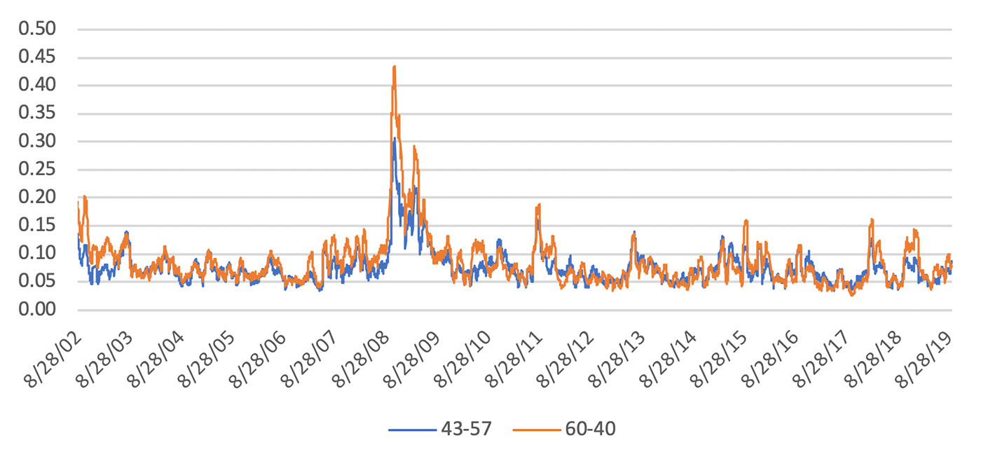
When we combine the two asset classes of stocks and bonds, we significantly reduce volatility. The average volatility of the 60-40 allocation is 9.70%, and the 43-57 allocation is 8.23%, about 15% lower. Both are shown in Figure 7.

But a peak volatility of 30% can still be too high for most investors.

Source: Market data, P. Kaufman

So far, we have only looked at passive portfolios of stocks and bonds. To reduce extreme risk, we will need to monitor that risk and rebalance the portfolio in a timely way. The method is called volatility stabilization. You cannot let the market control your risk, so this is a very important process.

First, decide the acceptable risk level for your portfolio. The industry standard is a target volatility of 12%. It means that 1 standard deviation of the daily returns is 12%. In other words, there is a 2.5% chance of losing 24% over the period of the tested data. Some institutions will set the target as low as 8%, which reduces the chance of a loss to 16%, but it also reduces the potential returns. Our example will use leveraged S&P 500 ETFs because we will need to be able to leverage up and down.

The concept is that, when volatility increases above our 12% target, we reduce our exposure. That is essentially the same as taking profits. Some analysts believe that, when volatility increases, we are making money and should continue holding the same position regardless of the volatility. But volatility is risk, and that works in your favor until it doesn’t! A client who is sensitive to risk will be delighted to see a one-day gain of 5% but not nearly as rational when it is a one-day loss of 5%.

Deleveraging may result in a small loss of return in exchange for a large reduction in risk. The biggest gain is when you increase leverage during a period of low volatility. Low-volatility periods tend to be when trend-following strategies make most of their money. If your target volatility is 12% and you expect to have a return of 15%, then when volatility drops to 6% your expected return falls to 7.5%. You are leaving half your gains on the table.

Using ETFs, there is an easy way to vary your leverage. Start with the triple-leverage S&P 500 ETF, SPXL, but only allocate one-third of your investment, leaving two-thirds in reserve. You will get the same returns as SPY. However, if volatility falls from 12% to 9%, you can double your position and still have one-third in reserve. If volatility falls to 6%, you can invest all of the money. It’s a simple solution to leveraging, and you will normally achieve the returns you expected.

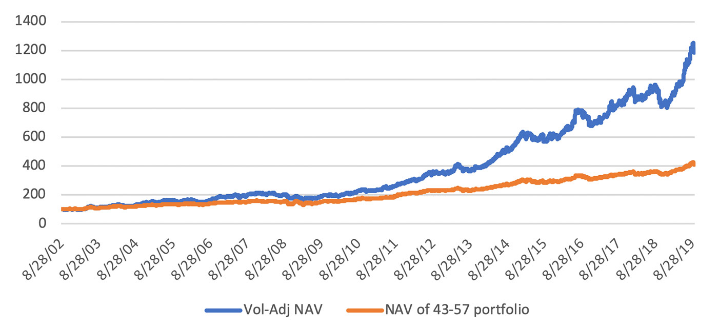
Figure 8 compares the basic 43-57 portfolio of stocks and bonds with the volatility-adjusted returns using the method just explained. Returns have increased by about 300%. While the absolute drawdowns look larger, the percentages are not.

Source: Market data, P. Kaufman

In the volatility-adjusted NAV (net asset value), the drawdown at the end of 2018 is only 16.5%, compared to the maximum drawdown of 23% that occurred on March 3, 2009.

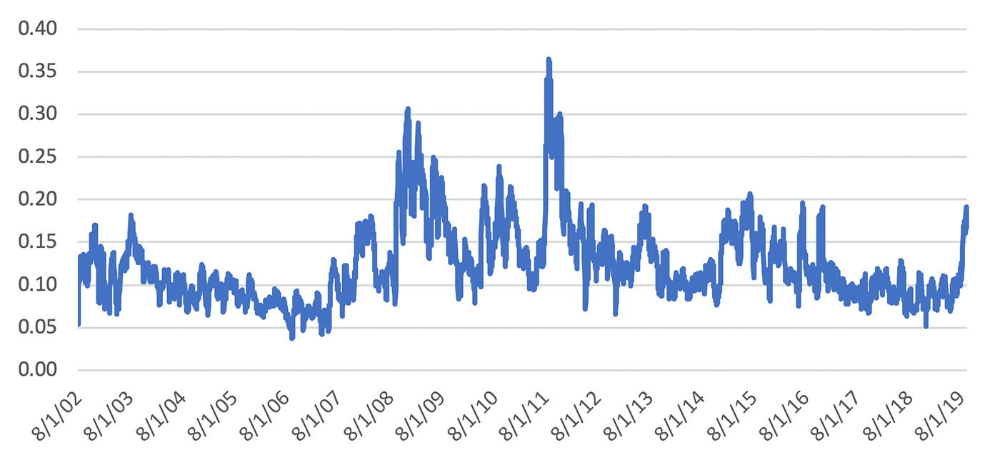
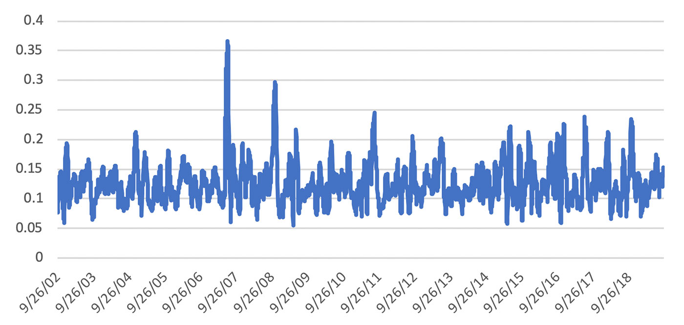
To give you a better idea of how volatility stabilization looks, Figures 9 shows the volatility of the portfolio after adjusting. This should be compared to Figure 6. The notable difference is that the periods of lower volatility, as shown in Figure 6, are now higher, and the general appearance is more uniform. The conclusion that we can draw is that long periods of profitability are missed because the portfolio is underleveraged; therefore, it cannot take advantage of the gains. It is an argument for leveraged ETFs or futures.

Source: Market data, P. Kaufman

Many investors and fund managers have decided that the trend has been fully exploited—that is, a strategy based on a moving average no longer works all that well. But that is not true.

The trend is the simplest of all technical tools, and the most reliable. It is not immune from drawdowns, but it seldom fails to improve results. A trend overlay is a way of applying conservation of capital. It takes small losses while sticking with the good moves.

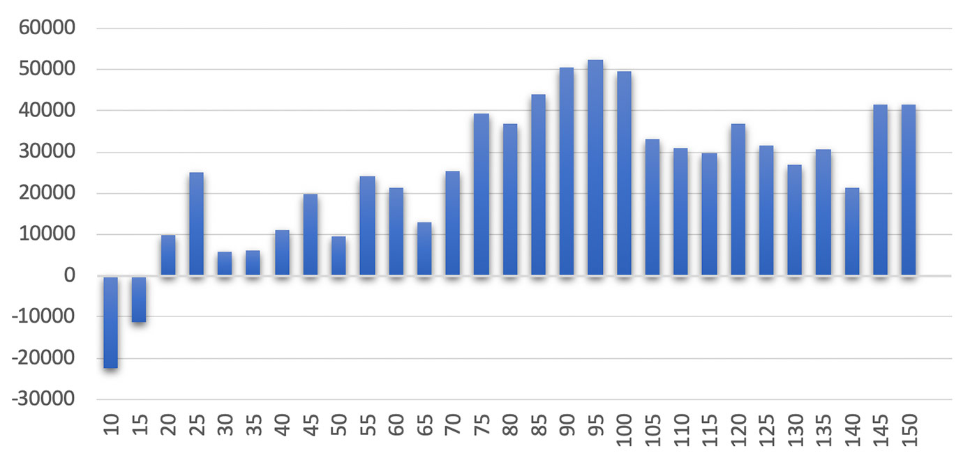
To show that the trend is a robust tool, we ran a test of moving averages with calculation periods from 10 days to 150 days, applied to SPY and TLT from 2002 through September 2019. The results are shown in Figures 10 and 11. The simple rules are that you go long when the moving average turns up and exit when it turns down.

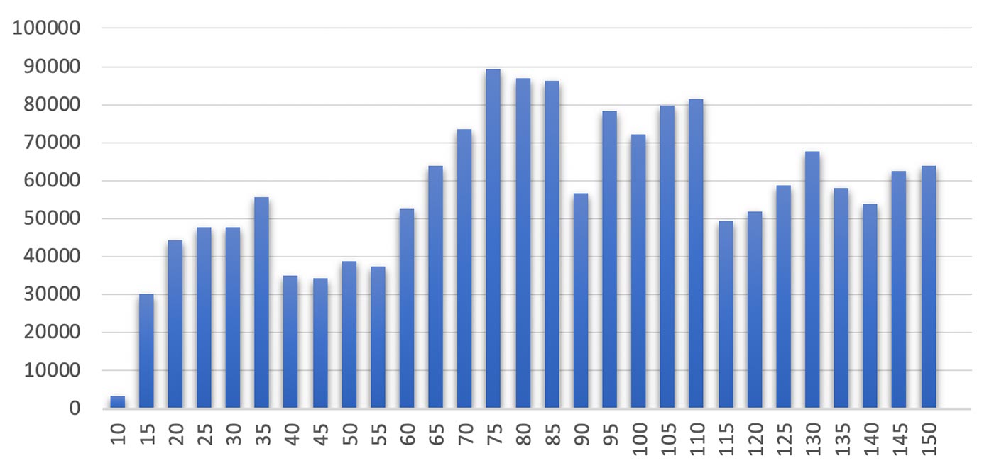
Note: Left-hand scale represents net profits.

Source: Market data, P. Kaufman

Note: Left-hand scale represents net profits.

Source: Market data, P. Kaufman

The tests show that the use of a moving-average strategy would have been profitable (long only) for both SPY and TLT for nearly all calculation periods. We will now apply it to the results of the 43-57 SPY-TLT portfolio, without volatility stabilization. Figure 12 compares the NAV of the portfolio with and without a 30-day moving-average trend.

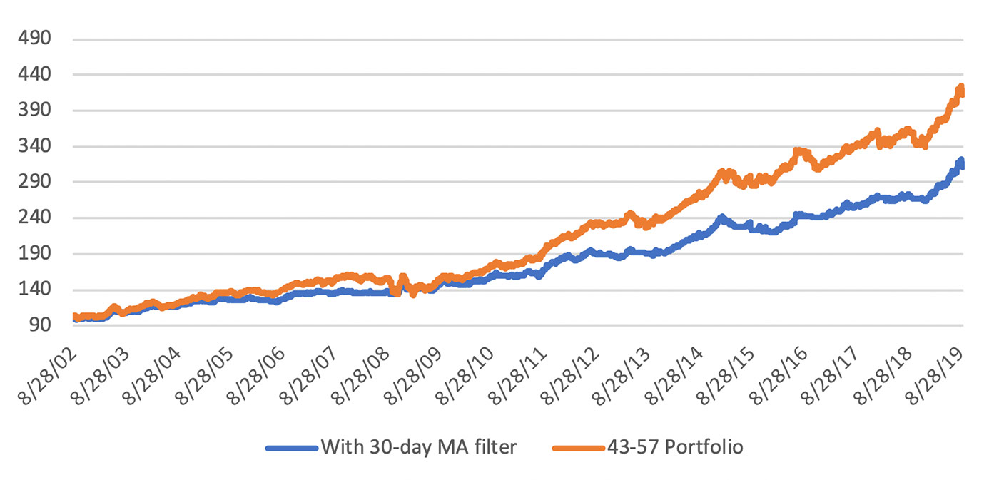
Source: Market data, P. Kaufman

From Figure 12 it appears that the trend causes an unacceptable drop in performance, but the chart can be deceiving. The return of the original 43-57 portfolio was 8.5% with a drawdown of 18.6%. The trend-filtered returns are 7.0% with a drawdown of 9.4%. That’s half the drawdown. You can always leverage these results by 2X and get a 14% return for the same drawdown as the original portfolio.

Risk management is now a high priority among many investors, especially those in or facing retirement. Many will accept far lower returns for a reduction in risk. This article has attempted to show a number of ways that risk may be better managed, without substantially reducing returns:

1. Allocating more to bonds and less to equities. (Note: There has been extensive commentary in the financial press on bond risk in the next rising-rate environment. Much of that is true. My answer is simply that this analysis includes environments of both rising and decreasing rates and the key is to focus on results over lengthy time periods and full market cycles.)
2. Managing risk using volatility stabilization.
3. Using a simple trend strategy overlay with your portfolio.
4. Using leveraged ETFs shows a dramatic improvement in both absolute returns and returns relative to risk.

The most improvement comes when you leverage up during periods when the volatility of your returns falls below your target. That’s when the market is doing its best and you are not benefiting at the level you expect. Adding a trend filter greatly reduced the drawdown at the cost of a modest reduction in return. This can be corrected with leveraged ETFs.

These methods all require some active participation and monitoring of performance, but the added risk control far outweighs the effort.

For those who do not have the time, inclination, or confidence to attempt this on their own, many of these tools are fundamentally at the heart of some very sophisticated strategies employed by third-party active investment management firms.

(For those who would like more information on using Solver and a spreadsheet that does the calculations for volatility stabilization, contact Perry Kaufman at [email protected].)